Jeremy Vachier
Theoretical Physicist | Associate Director Data Science
Absorbing Markov Chain Analysis for Predictive Maintenance
Understanding when equipment will fail is a fundamental challenge in predictive maintenance. Absorbing Markov chains provide a powerful mathematical framework to model equipment degradation and predict expected time to failure. This post explores the theory and implementation of a Python tool that computes expected steps to absorption from transient states.
→ View Full Implementation on GitHub
The Problem: Predicting Equipment Failure
Challenge: Equipment doesn’t fail instantaneously. It progressively deteriorates through intermediate health states before reaching complete failure.
Solution: Model equipment health as an absorbing Markov chain where:
- Transient states represent various degradation levels (healthy, slight wear, moderate damage, severe degradation)
- Absorbing state represents complete failure (a state that, once entered, cannot be left)
Goal: Compute the expected number of time steps (operating hours, cycles, etc.) before equipment transitions from its current state to failure.
Markov Chain Visualization
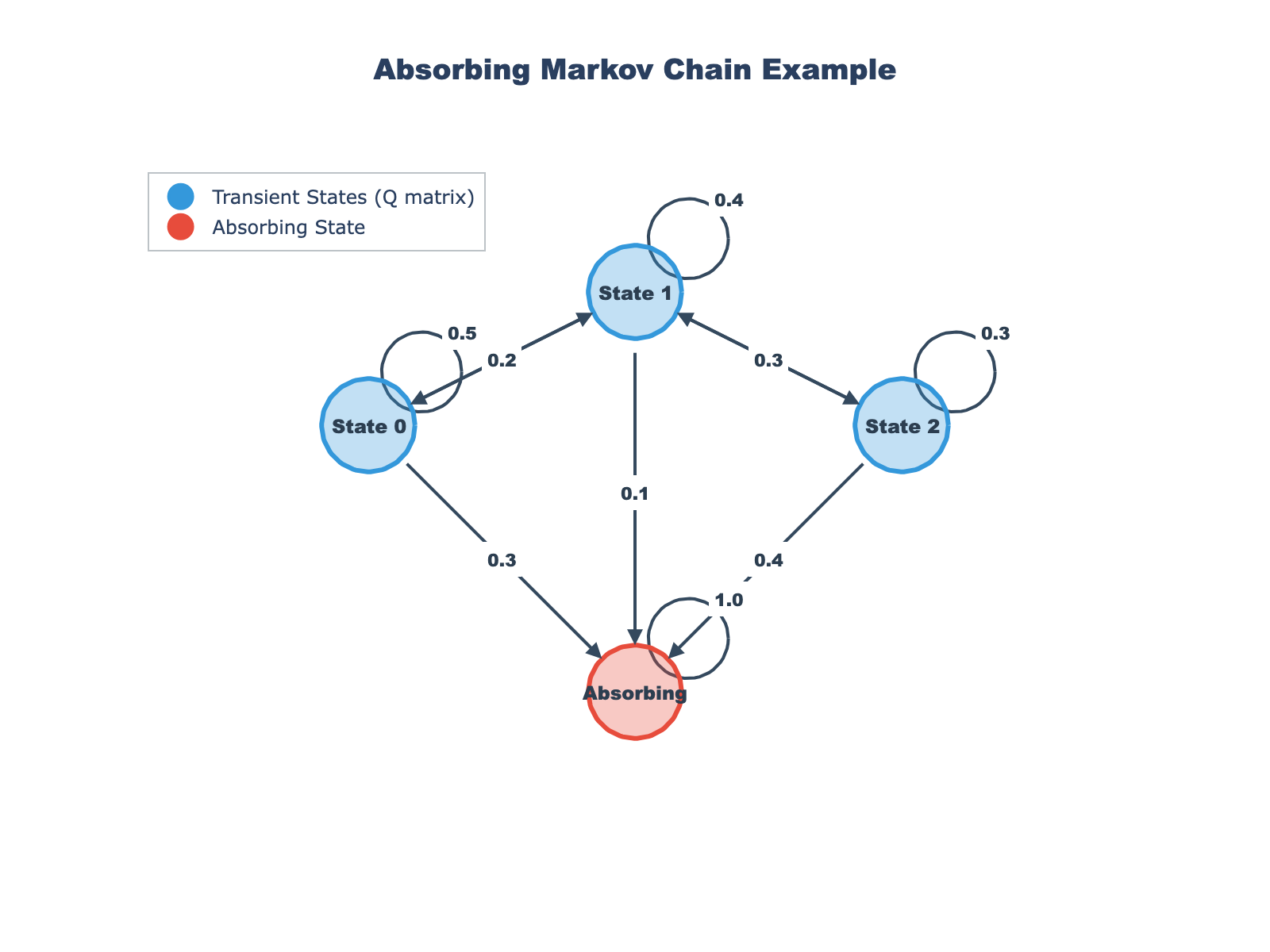
The diagram above shows an example absorbing Markov chain with transient states and absorbing states. The arrows indicate transition probabilities between states.
Part 1: The Drunkard’s Walk Analogy
The classic “drunkard’s walk” problem provides an intuitive understanding of absorbing Markov chains and their application to predictive maintenance.
The Story
A drunk person randomly walks between a bar and the sea. At each time step:
- They move one step toward the bar with probability $p$
- They move one step toward the sea with probability $1-p$
- If they reach the bar, they stay there (absorbing state)
- If they reach the sea, they fall in and cannot return (absorbing state)
Question: Starting from position $i$, how many steps on average before reaching either the bar or the sea?
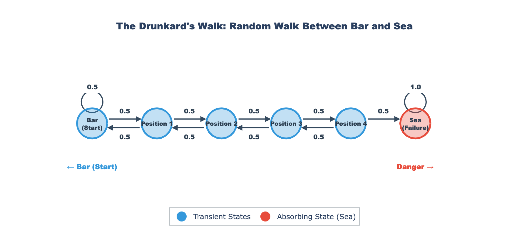
The Maintenance Analogy
The Bar represents perfect operating state (fully repaired or new equipment)
The Sea represents complete failure (equipment must be replaced)
Random steps represent the stochastic nature of equipment deterioration over time
Intermediate positions represent degradation states:
- Position 0: Perfect condition
- Position 1: Minor wear
- Position 2: Moderate degradation
- Position 3: Severe damage
- Position 4: Complete failure (sea)
Just as the drunkard can move both toward and away from the sea, equipment can:
- Degrade (move toward failure) through wear, stress, adverse conditions
- Improve slightly (move toward better states) through minor repairs, favorable operating conditions, or maintenance actions
This framework transforms qualitative notions of “equipment health” into quantitative predictions.
Part 2: Mathematical Framework
Absorbing Markov Chain Definition
An absorbing Markov chain is a Markov process containing:
- Transient states: States that can eventually be left (e.g., various degradation levels)
- Absorbing states: States that, once entered, cannot be left (e.g., complete failure)
Key property: From every transient state, there exists a path to at least one absorbing state.
Transition Matrix in Canonical Form
The transition matrix $P$ for an absorbing Markov chain can be written in canonical form:
\[P = \begin{bmatrix} Q & R \\ 0 & I \end{bmatrix}\]where:
- $Q$: $n \times n$ matrix of transient-to-transient transitions
- $R$: $n \times m$ matrix of transient-to-absorbing transitions
- $0$: $m \times n$ zero matrix (absorbing states don’t transition to transient states)
- $I$: $m \times m$ identity matrix (absorbing states stay in themselves)
Important constraint: Each row of $Q$ must sum to a value $\leq 1$, where the remainder $1 - \sum_j Q_{ij}$ represents the probability of transitioning to absorbing states.
The Fundamental Matrix
The fundamental matrix $N$ is defined as:
\[N = (I - Q)^{-1}\]where $I$ is the $n \times n$ identity matrix.
Interpretation: The element $N_{ij}$ represents the expected number of times the chain visits transient state $j$, starting from transient state $i$, before absorption.
Why does this work? Consider the infinite series:
\[N = I + Q + Q^2 + Q^3 + \cdots = \sum_{k=0}^{\infty} Q^k\]Each term $Q^k$ represents the probability of being in each transient state after exactly $k$ steps. Since $Q$ has row sums $< 1$, the series converges to $(I - Q)^{-1}$.
Expected Steps to Absorption
Multiplying the fundamental matrix by the vector of ones gives the total expected steps:
\[\mathbf{t} = N \times \mathbf{1}\]where $\mathbf{1} = (1, 1, \ldots, 1)^T$ is the $n \times 1$ vector of ones.
Interpretation: The element $t_i = \sum_j N_{ij}$ represents the expected total number of steps to reach an absorbing state, starting from transient state $i$.
Mathematical proof sketch:
- Let $t_i$ be the expected steps to absorption from state $i$
- From state $i$, we take one step, then continue from the next state
- This gives: $t_i = 1 + \sum_j Q_{ij} t_j$
- In matrix form: $\mathbf{t} = \mathbf{1} + Q\mathbf{t}$
- Solving: $\mathbf{t} - Q\mathbf{t} = \mathbf{1} \Rightarrow (I - Q)\mathbf{t} = \mathbf{1} \Rightarrow \mathbf{t} = (I-Q)^{-1}\mathbf{1} = N\mathbf{1}$
Part 3: Implementation
The Python implementation provides a clean interface for analyzing absorbing Markov chains.
Configuration Format
Define your Q matrix in config.json:
{
  "Q_matrix": [
    [0.5, 0.3, 0.1],
    [0.2, 0.4, 0.1],
    [0.3, 0.3, 0.1]
  ],
  "state_names": ["State 0", "State 1", "State 2"]
}
Interpretation of this example:
- 3 transient states (State 0, State 1, State 2)
- From State 0: 50% stay in State 0, 30% go to State 1, 10% go to State 2, 10% go to absorption
- From State 1: 20% go to State 0, 40% stay in State 1, 10% go to State 2, 30% go to absorption
- From State 2: 30% go to State 0, 30% go to State 1, 10% stay in State 2, 30% go to absorption
Core Algorithm
The implementation follows three main steps:
Step 1: Load and Validate Q Matrix
def load_config(config_path: str = "config.json") -> tuple[np.ndarray, list[str]]:
    """
    Load the Q matrix and state names from a JSON configuration file.

    Args:
        config_path: Path to the JSON configuration file

    Returns:
        tuple: (Q_matrix as numpy array, list of state names)

    Raises:
        FileNotFoundError: If config file doesn't exist
        ValueError: If Q matrix is invalid
    """
    config_file = Path(config_path)

    if not config_file.exists():
        raise FileNotFoundError(f"Configuration file not found: {config_path}")

    with open(config_file, "r") as f:
        config = json.load(f)

    Q_matrix = np.array(config["Q_matrix"], dtype=float)
    state_names = config.get(
        "state_names", [f"State {i}" for i in range(len(Q_matrix))]
    )

    # Validate Q matrix
    validate_q_matrix(Q_matrix)

    return Q_matrix, state_names


def validate_q_matrix(Q: np.ndarray) -> None:
    """
    Validate that Q is a valid transient-to-transient transition matrix.

    Args:
        Q: The Q matrix to validate

    Raises:
        ValueError: If Q matrix is invalid
    """
    if Q.ndim != 2:
        raise ValueError("Q matrix must be 2-dimensional")

    if Q.shape[0] != Q.shape[1]:
        raise ValueError("Q matrix must be square")

    if np.any(Q < 0):
        raise ValueError("Q matrix cannot contain negative values")

    if np.any(Q > 1):
        raise ValueError("Q matrix cannot contain values greater than 1")

    row_sums = Q.sum(axis=1)
    if np.any(row_sums > 1.0 + 1e-10):  # Small tolerance for floating point errors
        raise ValueError(f"Q matrix row sums must be ≤ 1.0 (found: {row_sums})")
Step 2: Compute Fundamental Matrix
def compute_fundamental_matrix(Q: np.ndarray) -> np.ndarray:
    """
    Compute the fundamental matrix N = (I - Q)^(-1).

    Args:
        Q: The transient-to-transient transition matrix

    Returns:
        The fundamental matrix N

    Raises:
        np.linalg.LinAlgError: If (I - Q) is singular
    """
    identity = np.eye(len(Q))
    N = np.linalg.inv(identity - Q)
    return N
Step 3: Calculate Expected Steps
def compute_expected_steps(N: np.ndarray) -> np.ndarray:
    """
    Compute expected number of steps to absorption for each transient state.

    Args:
        N: The fundamental matrix

    Returns:
        Vector of expected steps for each transient state
    """
    ones = np.ones(len(N))
    t = N @ ones
    return t
Example Output
Q matrix (transient to transient transitions):
[[0.5 0.3 0.1]
 [0.2 0.4 0.1]
 [0.3 0.3 0.1]]

Fundamental matrix N = (I - Q)^(-1):
[[3.75 2.5 1.25]
 [2.5 3.33 1.25]
 [2.5 2.5 2.08]]

Expected number of steps to absorption for each transient state:
State 0: 7.5000 steps
State 1: 7.0833 steps
State 2: 7.0833 steps
Interpretation:
- Starting from State 0, equipment will take on average 7.5 time units to reach failure
- Starting from State 1 or State 2, equipment will take approximately 7.08 time units to reach failure
- The fundamental matrix reveals that from State 0, the system expects to visit State 0 itself 3.75 times, State 1 about 2.5 times, and State 2 about 1.25 times before absorption
Part 4: Applications in Predictive Maintenance
Key Insights for Maintenance Strategy
1. Expected Time to Failure
The fundamental matrix allows us to compute the expected number of time steps (operating hours, cycles, production batches) before equipment transitions from its current health state to failure.
Example: If a machine is currently in “moderate degradation” (State 2) and each state represents 100 operating hours, the expected time to failure is:
\[\text{Expected time to failure} = 7.0833 \times 100 = 708.33 \text{ hours}\]2. Intervention Planning
By knowing expected steps to absorption, maintenance teams can schedule interventions before critical failure occurs.
Decision rule:
- If expected steps $> $ safety threshold: continue monitoring
- If expected steps $\leq$ safety threshold: schedule preventive maintenance
3. Cost Optimization
Understanding transition probabilities helps balance preventive maintenance costs against failure costs:
\[\text{Total expected cost} = C_{\text{preventive}} \times P(\text{preventive}) + C_{\text{failure}} \times P(\text{failure})\]Where:
- $C_{\text{preventive}}$ is the cost of scheduled maintenance
- $C_{\text{failure}}$ is the cost of unplanned failure (typically much higher)
- Transition probabilities determine optimal intervention timing
4. Risk-Based Prioritization
Different starting states yield different expected times to failure, enabling risk-based maintenance prioritization:
High priority: Equipment in states with low expected steps to absorption
Medium priority: Equipment in states with moderate expected steps
Low priority: Equipment in states with high expected steps (near-perfect condition)
Estimating Transition Probabilities from Data
In practice, the Q matrix is estimated from historical data:
Method 1: Direct observation \(Q_{ij} = \frac{\text{Number of transitions from state } i \text{ to state } j}{\text{Total transitions from state } i}\)
Method 2: Maximum likelihood estimation
For continuous-time Markov chains with state monitoring data
Method 3: Bayesian inference
When data is sparse, incorporate prior knowledge about degradation patterns
Part 5: Practical Considerations
State Definition
Challenge: How do you define transient states for real equipment?
Approaches:
- Sensor thresholds: Vibration levels, temperature zones, pressure ranges
- Degradation metrics: Remaining useful life percentages (100%, 75%, 50%, 25%)
- Inspection grades: Visual inspection classifications (A, B, C, D, F)
- Performance metrics: Efficiency levels, throughput rates, quality scores
Time Discretization
The Markov chain assumes discrete time steps. Choose the time granularity based on:
- Monitoring frequency (hourly, daily, per cycle)
- Degradation rate (slow vs. fast deteriorating equipment)
- Decision-making horizon (when can interventions be scheduled)
Model Validation
Validate the model by:
- Backtesting: Compare predicted vs. actual time to failure on historical data
- Cross-validation: Train on one subset of equipment, test on another
- Residual analysis: Check if prediction errors are random (model is well-specified)
Limitations
Markov assumption: Future state depends only on current state, not history
This may not hold if:
- Degradation exhibits memory effects (previous stress affects future degradation rate)
- Operating conditions change over time (seasonal patterns, usage intensity)
Stationary assumption: Transition probabilities don’t change over time
This may not hold if:
- Equipment ages (degradation accelerates)
- Maintenance practices improve (better preventive care)
- Operating environment changes (new production processes)
Solutions:
- Use semi-Markov chains if dwell times matter
- Use hidden Markov models if states are not directly observable
- Use time-inhomogeneous Markov chains if probabilities change over time
Part 6: Extensions and Advanced Topics
Multi-Absorbing State Chains
Real systems may have multiple failure modes:
- Mechanical failure (absorbing state 1)
- Electrical failure (absorbing state 2)
- Software fault (absorbing state 3)
The matrix $R$ in the canonical form reveals the probability of absorption into each specific failure mode:
\[B = NR\]where $B_{ij}$ is the probability of absorbing into state $j$ starting from transient state $i$.
Variance of Absorption Time
The fundamental matrix also allows computing the variance of time to absorption:
\[\text{Var}(T_i) = (2N - I)t - t^2\]This quantifies uncertainty in the prediction, enabling risk-adjusted maintenance planning.
Continuous-Time Markov Chains
For equipment monitored continuously, use continuous-time Markov chains (CTMCs), also known as jump Markov processes. Here, $Q$ is the infinitesimal generator matrix (rate matrix), where off-diagonal elements $Q_{ij} \geq 0$ represent transition rates and rows sum to zero.
The fundamental matrix for absorbing CTMCs is $N = (-Q_T)^{-1}$, where $Q_T$ is the transient-to-transient block of the generator. Expected time to absorption remains $\mathbf{t} = N\mathbf{1}$, now in continuous time units.
For a detailed treatment of continuous-time stochastic processes, see Vachier (2022).
Implementation Details
Technologies:
- Python 3.13+
- NumPy 2.0.0+ for matrix operations
- JSON for configuration management
- uv for dependency management
Project Structure:
absorbing-markov-chain/
├── main.py              # Core implementation
├── config.json          # Q matrix configuration
├── pyproject.toml       # Project dependencies
└── README.md            # Documentation
Usage:
# Install dependencies
uv sync

# Run analysis
uv run main.py
View the complete implementation on GitHub →
Key Takeaways
- Absorbing Markov chains provide a rigorous mathematical framework for modeling equipment degradation and predicting failure
- The fundamental matrix transforms state transition probabilities into actionable maintenance insights
- Expected steps to absorption enable data-driven maintenance scheduling that balances cost and risk
- The drunkard’s walk analogy makes the abstract mathematics intuitive for understanding stochastic degradation processes
- Real-world applications require careful state definition, parameter estimation, and model validation to ensure predictions are reliable
Mathematical Summary
Core equations:
Fundamental matrix:
\[N = (I - Q)^{-1} = \sum_{k=0}^{\infty} Q^k\]Expected steps to absorption:
\[\mathbf{t} = N\mathbf{1}\]Absorption probabilities:
\[B = NR\]Variance of absorption time:
\[\text{Var}(T_i) = (2N - I)t - t^2\]References
Mathematical foundations:
- Kemeny, J. G., & Snell, J. L. (1976). Finite Markov Chains. Springer-Verlag.
- Norris, J. R. (1998). Markov Chains. Cambridge University Press.
Stochastic processes:
- Vachier, J. (2020). Nonequilibrium Statistical Mechanics: Collective Behavior of Active Particles. PhD Thesis, Georg-August-Universität Göttingen. https://ediss.uni-goettingen.de/handle/21.11130/00-1735-0000-0005-136F-A
- Vachier, J., et al. (2020). Social cooperativity of bacteria during reversible surface attachment in young biofilms: a quantitative comparison of Pseudomonas aeruginosa PA14 and PAO1. mBio, 10(6), e02644-19. https://doi.org/10.1128/mbio.02644-19
Citation
If you use this tool in your research or project, please cite:
@software{absorbing_markov_chain,
  title = {Absorbing Markov Chain Analysis},
  author = {Vachier, J.},
  year = {2025},
  url = {https://github.com/jvachier/Absorbing-Markov-chain}
}
Tags: #PredictiveMaintenance #MarkovChains #Reliability #Mathematics #Python #NumPy #DataScience
License: MIT
Created: December 2025
Have questions about implementing absorbing Markov chains for your maintenance application? Feel free to reach out or open an issue on the GitHub repository!