Physics-Informed Neural Networks for Langevin Dynamics

From Langevin Trajectories to Physics-Constrained Density Prediction

This post walks through what appears to be a straightforward example of a physics-informed machine learning pipeline, though it turns out to be less straightforward than expected. The setup is rooted in the Langevin equation, the same stochastic differential equation that has been a constant thread through my research. The full implementation is available on GitHub.

The central question is: given particle trajectories generated by a known stochastic process, can a neural network learn not just the instantaneous probability density, but also the dynamical law that governs how that density evolves forward in time, without any further simulation data?

→ View Full Implementation on GitHub

Physics Background

The position $x(t)$ of a particle follows the Langevin equation [3]:

\[\frac{d}{dt}x = v_s + \sqrt{2 D_t} \, \xi(t),\]

where $v_s$ is the drift velocity, $D_t$ is the translational diffusion coefficient, and $\langle \xi(t’) \xi(t) \rangle = \delta(t’ - t)$ is a Gaussian white noise.

The Langevin equation allows us to express the probability of finding a particle at position $x$ at a given time $t$ through the Fokker–Planck equation [4], which describes the evolution of the probability density function $P(x, t \mid x_0, t_0)$, with the initial condition $P(x, t{=}t_0 \mid x_0, t_0) = \delta(x - x_0)$. To simplify the notation, we write $P(x, t) = P(x, t \mid x_0, t_0)$ and arrive at:

\[\frac{\partial P}{\partial t} = -v_s \frac{\partial P}{\partial x} + D_t \frac{\partial^2 P}{\partial x^2},\]

which has the analytic solution:

\[P(x,t) = \frac{1}{\sqrt{4\pi D_t (t - t_0)}} \exp\!\left(-\frac{(x - x_0 - v_s (t - t_0))^2}{4 D_t (t - t_0)}\right).\]

This analytic solution is exact. It serves as the ground truth throughout the project and is what the neural network is trained to reproduce and eventually to propagate forward in time without simulation.

The Pipeline

The project is structured as two coupled modules: a C++17/OpenMP Euler–Maruyama simulator that generates trajectory data, and a TensorFlow/Keras neural network pipeline that consumes it.

C++ simulator (Euler–Maruyama)
    ↓  simulation.bin  (~38 MB, 10⁵–10⁶ trajectories)
data_preparation  →  prepdata_from_binary.parquet
data_analytic     →  analytic_data.parquet  (Fokker–Planck Gaussian)
neural_network    →  PDF predictor  (histogram + time → P(x,t))
                  →  FP propagator  (P(x,t) + Δt → P(x, t+Δt))
rollout           →  autoregressive future-state prediction

C++ Simulation: Euler–Maruyama Integration

The simulator integrates the Langevin equation using the Euler–Maruyama scheme:

\[x(t + \Delta t) = x(t) + v_s \Delta t + \sqrt{2 D_t \Delta t} \, \eta,\]

where $\eta \sim \mathcal{N}(0, 1)$. The loop over $N_\text{particles} \times N_\text{steps}$ is parallelised with OpenMP across available cores and writes a compact binary output that the Python side reads via a Parquet conversion step.

A Dockerfile is provided for the simulation layer, particularly useful in CI or on machines where the host compiler does not support OpenMP out of the box.

All physical parameters, $v_s$, $D_t$, $\Delta t$, number of particles, number of time steps, are kept in a plain-text parameter.txt, synchronized with settings.toml on the Python side. Keeping physical parameters in one place and in physical units (rather than buried in code) is a discipline I have come to enforce after too many debugging sessions.

The Neural Networks

PDF Predictor

The first model learns the map:

\[\text{histogram}(x, t),\; t \;\longrightarrow\; P(x, t)\]

At each training time-step, the histogram of Langevin simulation positions and the current time are fed to the network, which predicts the smooth probability density. The training target is the analytic Fokker–Planck Gaussian, the network is trained to smooth the histogram while respecting the known physical solution.

This is a regression problem on a fixed spatial grid of n_bins histogram bins. The physics enters not through a residual penalty term at this stage, but through the choice of training target: the Fokker–Planck solution rather than the raw histogram. The network learns to associate temporal context $t$ with the correct spreading and drifting Gaussian.

Training uses a fraction train_test_split of all time-steps; the remainder forms the test set. Generalisation to held-out time-steps unseen during training confirms that the model has learned the temporal evolution rule rather than memorised individual frames.

Fokker–Planck Propagator

The second model is where the physics-informed constraint enters explicitly. It learns the map:

\[P(x, t) + \Delta t \;\longrightarrow\; P(x, t + \Delta t)\]

The propagator is trained with a curriculum on prediction gap: multi_step controls the maximum $\Delta t$ (in simulation steps) presented during training, ramping up the difficulty from single-step to multi-step prediction. The Fokker–Planck residual, the PDE evaluated at the network’s output, is added to the loss with a tunable weight $\lambda$:

\[\mathcal{L} = \mathcal{L}_\text{data} + \lambda \, \mathcal{L}_\text{FP}\]

where $\mathcal{L}_\text{FP}$ measures how far the predicted density deviates from satisfying

\[\frac{\partial P}{\partial t} = -v_s \frac{\partial P}{\partial x} + D_t \frac{\partial^2 P}{\partial x^2}\]

at the output grid points. This is the physics-informed component: the network is penalised not just for being far from the training data, but for violating the differential equation.

At inference, the rollout uses analytic teacher forcing: rather than feeding back the network’s own previous output at each step, the input histogram is reconstructed from the analytically known mean and variance of the Gaussian at that step. This is a deliberate engineering choice. In a fully autoregressive rollout, the softplus activation introduces a small floor on the output distribution tails, which inflates the predicted variance and compounds over steps. Teacher forcing sidesteps this by keeping the input always within the training distribution, so the network acts as a one-step corrector rather than a fully autonomous propagator. Closing the loop between the network’s output and its next input, without analytic scaffolding, is the natural next step for this project.

Results

Figure 1, PDF Predictor: Training Set

The neural network (red) learns to reproduce the analytic Fokker–Planck Gaussian (blue) from the Langevin simulation histogram (orange) on training time-steps. The network correctly learns to smooth the histogram, placing its prediction close to the analytic curve rather than fitting the statistical fluctuations.

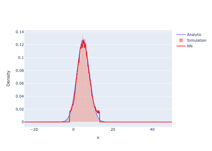
Figure 1: PDF predicted by the neural network (red) vs. the analytic solution (blue) and simulation histogram (orange) at a representative training time-step.

Figure 2, PDF Predictor: Test Set

Generalisation holds on held-out time-steps. The model has learned the temporal structure of the Gaussian, its drift and diffusive spreading, rather than memorising individual snapshots.

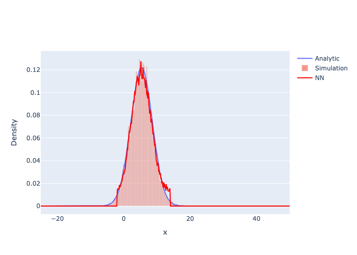
Figure 2: Same comparison on a held-out test time-step, confirming generalisation beyond the training distribution.

Figure 3, Propagator: Rollout with Analytic Teacher Forcing

The physics-constrained propagator predicts the PDF at five future times, $\tau \approx 2.5 \to 10$. At each step, the input is a Gaussian reconstructed from the analytically known mean and variance, analytic teacher forcing, rather than the network’s own previous output. The dashed red curve tracks the analytic Gaussian (blue) closely across the full rollout window.

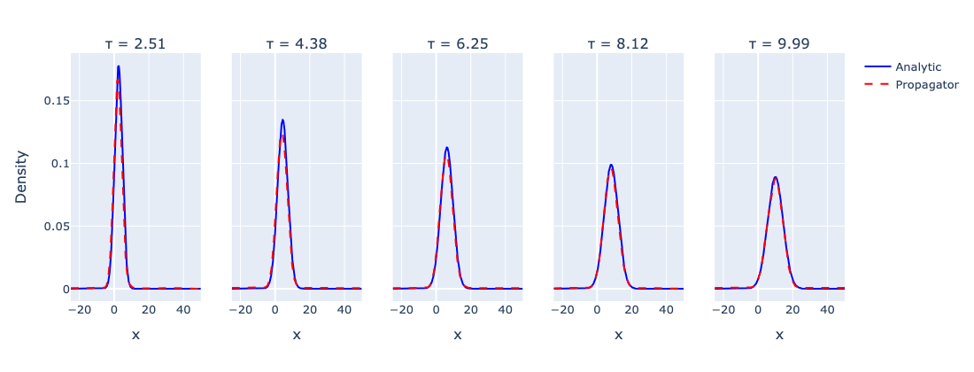
Figure 3: Rollout of the Fokker–Planck propagator (dashed red) at five future snapshots using analytic teacher forcing, compared to the analytic Gaussian (blue).

The result confirms that the network has learned a valid one-step map consistent with the Fokker–Planck equation. The open question, whether the network can sustain accurate rollout from its own output without analytic scaffolding, is the natural next step.

Engineering Notes

A few implementation choices worth making explicit.

Binary I/O over CSV. The simulator writes simulation.bin in binary format. At 38 MB for $10^5$–$10^6$ trajectories, reading binary and converting once to Parquet is considerably faster than parsing CSV at every run. This matters when you are iterating on the ML pipeline and do not want to re-run the simulation each time.

Decoupled configuration. Physical parameters ($v_s$, $D_t$, $\Delta t$) live in parameter.txt (C++ side) and settings.toml (Python side). The [physics] section of settings.toml must match parameter.txt exactly, no magic constants buried in code. This pattern has saved me from subtle bugs where the simulation and the analytic solution were computed with different parameter values.

Interactive figures. All plots are written as both .html (Plotly interactive) and .png (static). The interactive version is useful for inspecting the rollout frame by frame during development.

uv for dependency management. The Python environment uses uv sync against a pyproject.toml. Reproducible environments matter, especially when you want the CI badge to mean something.

Personal Context

The Langevin equation and the Fokker–Planck equation have been a constant thread through my research. An earlier paper solved the Fokker–Planck equation analytically for a sedimenting active Brownian particle in three dimensions under gravity, a considerably harder geometry than the 1D case here, requiring a full treatment of translational and rotational noise [1]. The same stochastic framework later appeared in a very different setting: biological particles embedded in ice near the melting point, driven by thermomolecular pressure gradients through interfacial premelting [2]. The physics differs entirely, but the mathematical structure, Langevin equation, Fokker–Planck evolution, analytic solution as ground truth, is identical.

That continuity is what makes this project feel natural. The question it asks is the inversion of what I spent years doing analytically: instead of deriving the probability density from the stochastic equation, can a neural network learn to propagate the density forward from data alone, constrained by knowledge of the governing PDE? In the 1D case with constant coefficients, the analytic solution exists and serves as a clean benchmark. In systems with confinement, spatially varying diffusivity, or active self-propulsion, it does not, and that is where this approach becomes genuinely useful.

References

[1] Vachier, J. & Mazza, M. G. (2019). Dynamics of sedimenting active Brownian particles. The European Physical Journal E, 42, 11. https://doi.org/10.1140/epje/i2019-11770-6

[2] Vachier, J. & Wettlaufer, J. S. (2022). Premelting controlled active matter in ice. Physical Review E, 105, 024601. https://doi.org/10.1103/PhysRevE.105.024601

[3] Langevin, P. (1908). Sur la théorie du mouvement brownien. C. R. Acad. Sci., 146, 530–533.

[4] Risken, H. (1989). The Fokker–Planck Equation: Methods of Solution and Applications (2nd ed.). Springer.