Jeremy Vachier
Theoretical Physicist | Associate Director Data Science
From Keywords to Semantics: A Technical Guide to Text Retrieval
From Exact Matching to Neural Encoders
Methods in information retrieval: from classical keyword matching to neural encoders trained with contrastive objectives. Each method is presented with its core equations, the paper that introduced it, and the intuition behind the design choices.
This post accompanies two Kaggle notebooks and a published synthetic dataset where these methods are implemented from scratch and benchmarked on a synthetic industrial maintenance dataset:
- Retrieval from Scratch: BM25, MLM pre-training, and SimCSE on MS MARCO and industrial text
- Hard Negative Mining for Dense Retrieval: a counterintuitive finding on when harder negatives hurt
- Industrial Maintenance Synthetic Data — generator on GitHub, dataset on HuggingFace and Kaggle
Why retrieval matters
Text retrieval is the problem of finding the most relevant documents in a large corpus given a query. It sits at the core of search engines, question-answering systems, and Retrieval-Augmented Generation (RAG) pipelines. The method you choose has a dramatic effect on what gets returned and the right choice depends on the nature of your queries and your corpus.
This post walks through five retrieval systems in order of increasing semantic sophistication: BM25, MLM-only encoders, unsupervised SimCSE, supervised SimCSE with hard negative mining, and MiniLM.
Evaluation metrics
Let $\mathcal{Q}$ be a set of evaluation queries, and for each query $q \in \mathcal{Q}$ let $\mathcal{R}_q$ be its set of relevant documents. All metrics below assume a ranked list of $K$ retrieved documents for each query.
Mean Reciprocal Rank (MRR@K)
\[\text{MRR} = \frac{1}{|\mathcal{Q}|} \sum_{q \in \mathcal{Q}} \frac{1}{\text{rank}_q^*}\]where $\text{rank}_q^*$ is the rank position of the first relevant document for query $q$, or $\infty$ if no relevant document appears in the top $K$. A system that always places the relevant document first achieves MRR = 1.0; one that always places it second achieves MRR = 0.5. MRR is the natural metric for single-relevant retrieval — one correct answer per query.
Normalised Discounted Cumulative Gain (NDCG@K)
Let $\text{rel}_i \in {0, 1}$ denote the relevance of the document at rank position $i$. The Discounted Cumulative Gain at rank $K$:
\[\text{DCG@K} = \sum_{i=1}^{K} \frac{\text{rel}_i}{\log_2(i+1)}\]The $\log_2(i+1)$ denominator discounts documents appearing lower in the list: a relevant document at rank 1 contributes $1/\log_2(2) = 1.0$, at rank 2 contributes $1/\log_2(3) \approx 0.63$, at rank 10 contributes $1/\log_2(11) \approx 0.29$. Normalisation by the Ideal DCG (IDCG), the DCG achieved when all relevant documents are ranked first — gives:
\[\text{NDCG@K} = \frac{\text{DCG@K}}{\text{IDCG@K}}\]NDCG@10 is the standard metric on MS MARCO (Nguyen et al., 2016) and BEIR (Thakur et al., 2021).
Recall@K
\[\text{Recall@K} = \frac{\left|\left\{d \in \text{top-}K : d \in \mathcal{R}_q\right\}\right|}{|\mathcal{R}_q|}\]where the numerator counts relevant documents in the top-$K$ results and the denominator is the total number of relevant documents for the query. Recall@100 is standard for first-stage retrieval pipelines where a reranker acts on the top-$K$ candidates.
1. BM25 — Probabilistic keyword matching
BM25 (Robertson et al., 1994; Robertson & Zaragoza, 2009) is derived from the probabilistic relevance framework. It scores document $d$ for query $q$ as a sum over query terms $t \in q$:
\[\text{BM25}(q, d) = \sum_{t \in q} \text{IDF}(t) \cdot \frac{f(t, d) \cdot (k_1 + 1)}{f(t, d) + k_1 \cdot \left(1 - b + b \cdot \dfrac{|d|}{\text{avgdl}}\right)}\]where:
- $f(t, d)$ is the raw term frequency of token $t$ in document $d$
- $\lvert d \rvert$ is the number of tokens in document $d$
- $\text{avgdl}$ is the mean document length across the corpus
- $k_1 \in [1.2, 2.0]$ is the term frequency saturation parameter — as $f(t,d) \to \infty$, the score saturates at $k_1 + 1$, preventing a single high-frequency term from dominating
- $b \in [0, 1]$ is the length normalisation parameter — $b = 1$ gives full normalisation, $b = 0$ disables it
The IDF component penalises terms that appear in many documents:
\[\text{IDF}(t) = \log\!\left(\frac{N - n(t) + 0.5}{n(t) + 0.5} + 1\right)\]where $N$ is the total number of documents in the corpus and $n(t)$ is the number of documents containing term $t$.
BM25 has no understanding of meaning, only matching of tokens. A query and a document must share the exact same token to produce a non-zero score. This makes BM25 fast, interpretable, and highly effective when vocabulary is controlled. It fails the moment a query uses different words to express the same meaning.
2. Transformer encoders and MLM pre-training
To go beyond keyword matching, we need embeddings, fixed-size vector representations of text such that semantically similar texts produce geometrically close vectors. The standard approach is to train a transformer encoder (Vaswani et al., 2017) and use its pooled output as an embedding.
Transformer architecture
A transformer encoder maps an input sequence of $n$ tokens $\mathbf{x} = [x_1, \ldots, x_n]$ to contextual representations $\mathbf{H} \in \mathbb{R}^{n \times d}$, where $d$ is the model dimension. Each block applies multi-head self-attention:
\[\text{MultiHeadAttention}(\mathbf{H}) = \text{Concat}(\text{head}_1, \ldots, \text{head}_h)\,\mathbf{W}^O\] \[\text{head}_m = \text{softmax}\!\left(\frac{\mathbf{Q}_m\mathbf{K}_m^\top}{\sqrt{d_k}}\right)\mathbf{V}_m\]where $h$ is the number of attention heads, $d_k = d/h$ is the dimension per head, $\mathbf{W}^O \in \mathbb{R}^{d \times d}$ is the output projection, and for each head $m$:
\[\mathbf{Q}_m = \mathbf{H}\mathbf{W}_m^Q, \quad \mathbf{K}_m = \mathbf{H}\mathbf{W}_m^K, \quad \mathbf{V}_m = \mathbf{H}\mathbf{W}_m^V\]with learned projection matrices $\mathbf{W}_m^Q, \mathbf{W}_m^K, \mathbf{W}_m^V \in \mathbb{R}^{d \times d_k}$. The $\sqrt{d_k}$ scaling factor prevents dot products from entering the saturation region of softmax as dimension grows.
For retrieval, we produce a single embedding by masked mean pooling over non-padding token representations, followed by L2 normalisation:
\[\mathbf{e} = \frac{\text{MeanPool}\!\left(f_\theta(\mathbf{x})\right)}{\left\|\text{MeanPool}\!\left(f_\theta(\mathbf{x})\right)\right\|_2} \in \mathbb{R}^d\]where $f_\theta : \mathbb{R}^n \to \mathbb{R}^{n \times d}$ denotes the transformer encoder with parameters $\theta$. Cosine similarity between two L2-normalised embeddings reduces to their inner product: $\text{sim}(\mathbf{e}_1, \mathbf{e}_2) = \mathbf{e}_1^\top \mathbf{e}_2 \in [-1, 1]$. (For the geometric framework behind this construction — why L2 normalisation projects onto the unit hypersphere and why this matters for retrieval — see RAG as a Hilbert Space Problem.)
Masked Language Modelling (MLM)
To learn useful representations without labelled data, BERT (Devlin et al., 2019) introduces Masked Language Modelling. A random subset $\mathcal{M}$ of positions (15% of non-padding tokens) is replaced with a [MASK] token, producing the masked sequence $\tilde{\mathbf{x}}$. The model is trained to recover the original tokens:
where $P(x_i \mid \tilde{\mathbf{x}};\, \theta)$ is obtained by projecting the transformer output at position $i$ onto the vocabulary. To predict masked tokens correctly, the model must learn syntax, semantics, and long-range contextual dependencies,making MLM a powerful general-purpose pre-training objective.
After MLM pre-training on a domain corpus, the encoder has learned domain vocabulary and co-occurrence patterns. This allows it to handle abbreviations and identifiers that BM25 cannot: if “mtr” consistently co-occurs with “motor” in the training corpus, their representations will be geometrically close.
3. Unsupervised SimCSE — Why it fails on passages
SimCSE (Gao et al., 2021) proposes a self-supervised contrastive objective. The augmentation is minimal: pass the same input $\mathbf{x}$ through the encoder twice with independent dropout masks, producing two views $\mathbf{z} = f_\theta(\mathbf{x})$ and $\mathbf{z}^+ = f_\theta(\mathbf{x})$ with different dropout realisations. These form a positive pair; all other sentences in the batch serve as in-batch negatives.
The InfoNCE loss (Oord et al., 2018) for a batch of size $N$:
\[\mathcal{L}_{\text{SimCSE}} = -\frac{1}{N} \sum_{i=1}^{N} \log \frac{\exp\!\left(\text{sim}(\mathbf{z}_i,\, \mathbf{z}_i^+)\, /\, \tau\right)}{\displaystyle\sum_{j=1}^{N} \exp\!\left(\text{sim}(\mathbf{z}_i,\, \mathbf{z}_j^+)\, /\, \tau\right)}\]where $\tau > 0$ is a temperature hyperparameter controlling the sharpness of the distribution. The random baseline loss, if the model assigns uniform probability to all $N$ candidates, is $\ln(N)$. The contrastive accuracy, the fraction of steps where the correct positive has the highest similarity, should start near $1/N$ and increase as the model learns.
The method works well on short sentences (avg. ~15 tokens in the original paper). For a 15-token sentence, two forward passes with different dropout masks produce meaningfully different attention patterns, forcing content-based representations.
For long passages, the method collapses. The empirical signature is unambiguous: contrastive accuracy = 1.0 from the very first training step, regardless of batch size or temperature. The mechanism is most easily understood by noting that the mean-pooled embedding of a 70-token passage retains a strong token-overlap signature, two dropout views of the same passage share the same set of tokens, and their mean-pooled embeddings remain near-identical relative to the embeddings of unrelated passages in the batch. The model can match views by token overlap alone, trivially solving the contrastive task without learning attention-based semantics.
The fix is not hyperparameter tuning, it requires a fundamentally different positive pair construction.
4. Supervised SimCSE and hard negative mining
Supervised pairs
The supervised variant of SimCSE (Gao et al., 2021, §3.2) replaces dropout augmentation with explicit $(a, p, n)$ triplets: anchor $a$, positive $p$, and negative $n$. The positive is a genuinely different text semantically related to the anchor; the negative is semantically different. Let $\mathbf{z}_i^a$, $\mathbf{z}_i^p$, $\mathbf{z}_i^n$ be the L2-normalised embeddings of the $i$-th triplet. For a batch of size $B$:
\[\mathcal{L}_{\text{sup}} = -\frac{1}{B} \sum_{i=1}^{B} \log \frac{\exp\!\left(\text{sim}(\mathbf{z}_i^a,\, \mathbf{z}_i^p)\, /\, \tau\right)}{\displaystyle\sum_{j=1}^{B} \exp\!\left(\text{sim}(\mathbf{z}_i^a,\, \mathbf{z}_j^p)\, /\, \tau\right) + \sum_{j=1}^{B} \exp\!\left(\text{sim}(\mathbf{z}_i^a,\, \mathbf{z}_j^n)\, /\, \tau\right)}\]The denominator contains $2B$ candidates, $B$ positives and $B$ negatives. The random baseline is $\ln(2B)$. Because the positive and anchor are genuinely different texts, the model cannot solve this by token matching, it must learn semantic similarity.
Hard negative mining
Random negatives are often easy to distinguish from the anchor by vocabulary alone. Hard negatives are passages that are lexically similar to the anchor but semantically different, forcing finer-grained representations.
The mining procedure uses FAISS (Johnson et al., 2019) for approximate nearest-neighbour search. After initial pre-training, all $N$ passages are embedded and indexed. For each anchor $\mathbf{e}_i$, the top-$K$ most similar passages are retrieved. Passages sharing the anchor’s label are discarded; a hard negative $n_i$ is sampled from the remaining top candidates:
\[n_i = \text{sample}\!\left(\operatorname{top\text{-}}k\!\left\{d : \text{sim}(\mathbf{e}_i, \mathbf{e}_d) \text{ is large},\;\, \text{label}(d) \neq \text{label}(i)\right\}\right)\]IVFFlat indexing (Johnson et al., 2019) partitions the embedding space into $\text{nlist}$ Voronoi cells. At query time, only $\text{nprobe}$ cells are searched, reducing the effective search space from $N$ to approximately $N \cdot \text{nprobe}/\text{nlist}$ candidates. Setting $\text{nprobe} = \text{nlist}/4$ gives ~99% recall at roughly 10–20× the speed of exact search.
A practical caveat. When no hard candidate is found in the top $K$ (28.9% of anchors in our experiments), the implementation falls back to a random negative. This dilutes the comparison: the “hard-neg” condition is closer to a 71% hard + 29% random mixture than a pure-hard regime. Increasing $K$ or filtering more aggressively would reduce the fallback rate at the cost of mining time.
Hard negatives introduce a known tension in contrastive learning, sometimes called the local-vs-global trade-off: improving local discrimination, separating semantically similar but non-relevant passages, can come at the cost of global coverage. Robinson et al. (2021) propose a debiased sampling scheme designed to mitigate this trade-off; the trade-off itself is what their method targets.
5. MiniLM — Pre-training at scale
MiniLM (Wang et al., 2020) is a 6-layer, 22M parameter encoder obtained by distilling BERT through deep self-attention distillation. The all-MiniLM-L6-v2 checkpoint (released via Reimers & Gurevych, 2019’s sentence-transformers framework) takes this distilled backbone and fine-tunes it contrastively on over 1 billion sentence pairs - NLI datasets, paraphrase corpora, question-answer pairs, and web data - using in-batch negatives (Henderson et al., 2017). For a batch of $B$ query-document pairs $(\mathbf{q}_i, \mathbf{d}_i^+)$, where $\mathbf{q}_i$ and $\mathbf{d}_i^+$ are the L2-normalised embeddings of query $i$ and its paired positive document:
The result is a bi-encoder, where query and document are embedded independently and scored by cosine similarity, with semantic generalisation that domain-trained encoders cannot match. The gap between a domain-trained encoder and MiniLM is not primarily a matter of architecture or training objective. It is a matter of training data diversity.
Comparative results
The figure below summarises results from the two notebooks, comparing all five systems across three evaluation dimensions on a synthetic industrial maintenance dataset.
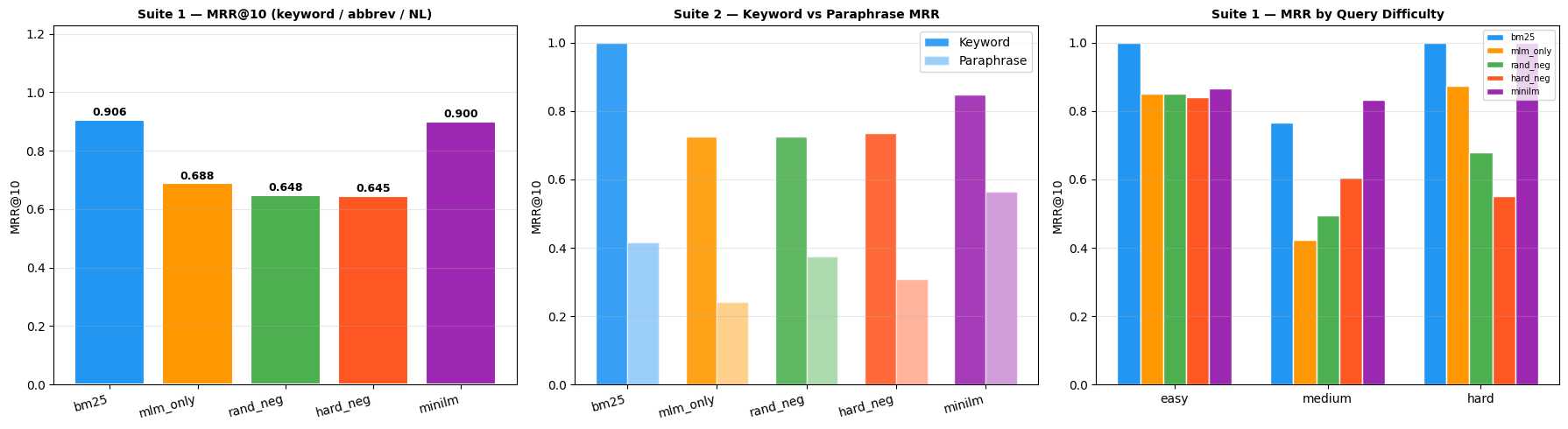
Left: MRR@10 on 20 baseline queries. Centre: keyword MRR vs paraphrase MRR. The gap between bars is the semantic gap. Right: MRR@10 by query difficulty.
Three findings stand out.
BM25 and MiniLM tie on the headline number but diverge in the tails. BM25 (0.906) and MiniLM (0.900) are essentially tied on baseline keyword queries, a small-vocabulary, highly structured corpus strongly favours exact-match retrieval. The two systems diverge sharply on edge cases: BM25 dominates bare activity codes (“CM02”) with MRR@10 = 1.0 where MiniLM scores 0.0, while MiniLM handles abbreviation-mixed queries (MRR@10 = 1.0) where BM25 fails completely on the literal mismatch.
The semantic gap reveals the limits of domain training. BM25 has a keyword-to-paraphrase gap of 0.586, it fails entirely when query and document share no tokens. Custom encoders reduce this gap modestly. MiniLM achieves a gap of 0.283, the benefit of 1 billion diverse training pairs.
Hard negatives improve cross-equipment discrimination but narrow semantic coverage. Rand-neg SimCSE achieves a smaller semantic gap (0.350) than hard-neg SimCSE (0.429), consistent with the local-vs-global trade-off in contrastive learning. Training on fine-grained distinctions narrows the semantic space the encoder explores. The size of this difference (~0.08 MRR over 10 paraphrase pairs) is suggestive rather than statistically robust. A single seed and a small evaluation set are real limitations, and the direction of the effect should be replicated before treating it as a load-bearing result. The cross-equipment improvement (+0.089 MRR over 8 queries) is in the expected direction and corroborates the trade-off interpretation.
Summary
| System | Keyword | Paraphrase | Domain identifiers | Speed |
|---|---|---|---|---|
| BM25 | Strong | Fails | Strong on bare codes; fails on mixed abbreviations | Very fast |
| MLM-only | Good | Weak | Weak on bare codes; modest on abbreviations | Fast |
| Rand-neg SimCSE | Moderate | Moderate | Weak | Fast |
| Hard-neg SimCSE | Moderate | Weak | Weak; best for cross-equipment discrimination | Fast |
| MiniLM | Strong | Strong | Fails on bare codes; strong on mixed abbreviations | Moderate |
No single system dominates. For a production pipeline: BM25 for first-stage retrieval, a strong bi-encoder like MiniLM for second-stage dense retrieval, optionally followed by a cross-encoder reranker on the top-$K$ candidates. A domain-trained encoder adds value specifically when the corpus contains structured identifiers or codes that general-purpose models have never seen and the choice between random and hard negatives should be made based on whether paraphrase generalisation or cross-instance discrimination is the bottleneck.
Limitations
- Relevance is assessed by keyword presence in the retrieved document, which systematically favours lexical systems and likely understates the paraphrase advantage of neural encoders.
- The evaluation suites are small (20 / 10 / 8 / 10 queries) and use a single random seed. Quantitative differences smaller than a few rank-position changes should not be over-interpreted.
- The industrial maintenance dataset is synthetic. The 2,346-token vocabulary is unusually small, partly because synthetic generators do not reproduce the long tail of real free-text maintenance notes. The generation procedure is available on GitHub for inspection or reuse.
- The hard-negative mining procedure falls back to a random negative for 28.9% of anchors. The hard-neg condition is therefore a hard/random mixture, not pure hard.
References
- Devlin, J., Chang, M. W., Lee, K., & Toutanova, K. (2019). BERT: Pre-training of deep bidirectional transformers for language understanding. NAACL-HLT.
- Gao, T., Yao, X., & Chen, D. (2021). SimCSE: Simple contrastive learning of sentence embeddings. EMNLP.
- Henderson, M., Al-Rfou, R., Strope, B., Sung, Y., Lukács, L., Guo, R., Kumar, S., Miklos, B., & Kurzweil, R. (2017). Efficient natural language response suggestion for smart reply. arXiv:1705.00652.
- Johnson, J., Douze, M., & Jégou, H. (2019). Billion-scale similarity search with GPUs. IEEE Transactions on Big Data, 7(3), 535–547.
- Nguyen, T., Rosenberg, M., Song, X., Gao, J., Tiwary, S., Majumder, R., & Deng, L. (2016). MS MARCO: A human generated machine reading comprehension dataset. NeurIPS Workshop on Cognitive Computation.
- Oord, A. V. D., Li, Y., & Vinyals, O. (2018). Representation learning with contrastive predictive coding. arXiv:1807.03748.
- Reimers, N., & Gurevych, I. (2019). Sentence-BERT: Sentence embeddings using Siamese BERT-networks. EMNLP.
- Robertson, S. E., Walker, S., Jones, S., Hancock-Beaulieu, M. M., & Gatford, M. (1994). Okapi at TREC-3. NIST TREC-3.
- Robertson, S., & Zaragoza, H. (2009). The probabilistic relevance framework: BM25 and beyond. Foundations and Trends in Information Retrieval, 3(4), 333–389.
- Robinson, J., Chuang, C. Y., Sra, S., & Jegelka, S. (2021). Contrastive learning with hard negative samples. ICLR.
- Thakur, N., Reimers, N., Rücklé, A., Srivastava, A., & Gurevych, I. (2021). BEIR: A heterogeneous benchmark for zero-shot evaluation of information retrieval models. NeurIPS Datasets and Benchmarks Track.
- Vaswani, A., Shazeer, N., Parmar, N., Uszkoreit, J., Jones, L., Gomez, A. N., Kaiser, Ł., & Polosukhin, I. (2017). Attention is all you need. NeurIPS.
- Wang, W., Wei, F., Dong, L., Bao, H., Yang, N., & Zhou, M. (2020). MiniLM: Deep self-attention distillation for task-agnostic compression of pre-trained transformers. NeurIPS.