Jeremy Vachier
Theoretical Physicist | Associate Director Data Science
The Same Encoder, a Different Distance: From Text Retrieval to Audio Anomaly Detection
Predictive maintenance traditionally relies on sensor data, such as temperature, pressure, vibration, and electrical current, to catch faults before they become failures. These signals are well understood, easy to record with standard instrumentation, and directly tied to the physical process being monitored. But they are not the only signal a machine emits. Every motor, pump, fan, and valve has an acoustic fingerprint: a characteristic sound pattern during normal operation that changes in detectable ways when something goes wrong.
Sound is rich, noninvasive, and cheap to record with a single microphone. The challenge is extracting fault information from it without labeled fault examples: in practice, faults are rare, and waiting to collect anomaly data before deploying a detector defeats the purpose. The question is: can a model trained exclusively on normal sounds learn to recognize when a recording no longer fits?
This post walks through three detector families on two datasets, in the order they were built. The first dataset is a single machine type under controlled conditions; the second scales to three machine types across multiple physical units with varying background noise. Reconstruction based models do well on the first and partially on the second. On the hardest machine type, they collapse to chance, and that failure motivates the embedding approach that closes the post.
The full implementations are in two Kaggle notebooks:
- Unsupervised Industrial Audio Anomaly Detection (MIMII pump dataset: Dense AE vs TransformerVAE)
- Unsupervised Audio Anomaly: AE, VAE, Transformer (DCASE 2020 Task 2: all three detector families)
Code and trained models: github.com/jvachier/industrial-audio-anomaly-detection · HuggingFace jvachier/dcase2020-task2-anomaly-detection
1. From raw audio to a feature representation
Before any model sees audio, the raw waveform must be converted into something a neural network can process. The standard pipeline for industrial sound is the log mel spectrogram.
A Short Time Fourier Transform (STFT) computes the power spectrum over short overlapping windows. Each window of $N = 512$ samples at 16 kHz gives a frequency resolution of $\Delta f = f_s / N = 31.25$ Hz/bin. The power at each bin is then projected onto a filterbank of triangular filters spaced on the mel scale, a perceptually motivated frequency axis that compresses the high frequency range and stretches the low frequency range:
\[m(f) = 2595\,\log_{10}\!\left(1 + \frac{f}{700}\right)\]Both constants come from fitting this curve to human pitch perception experiments (Stevens, Volkmann, and Newman, 1937): 700 Hz is the corner frequency below which the mel scale is approximately linear in $f$ and above which it turns logarithmic, matching how listeners judge pitch differences at low versus high frequencies; 2595 is a scaling constant chosen so that a 1000 Hz tone maps to 1000 mel by definition, $m(1000) = 2595\,\log_{10}(1 + 1000/700) \approx 1000$.
The result is a 2D array $S \in \mathbb{R}^{T \times F}$ where $T$ is the number of time frames and $F = 128$ is the number of mel bins: a compact, perceptually meaningful representation of the acoustic content.
The figure below shows a normal and an anomalous pump clip side by side. The structural difference is subtle: anomalous sounds do not look dramatically different to the eye, which is precisely why simple thresholding on raw audio does not work.
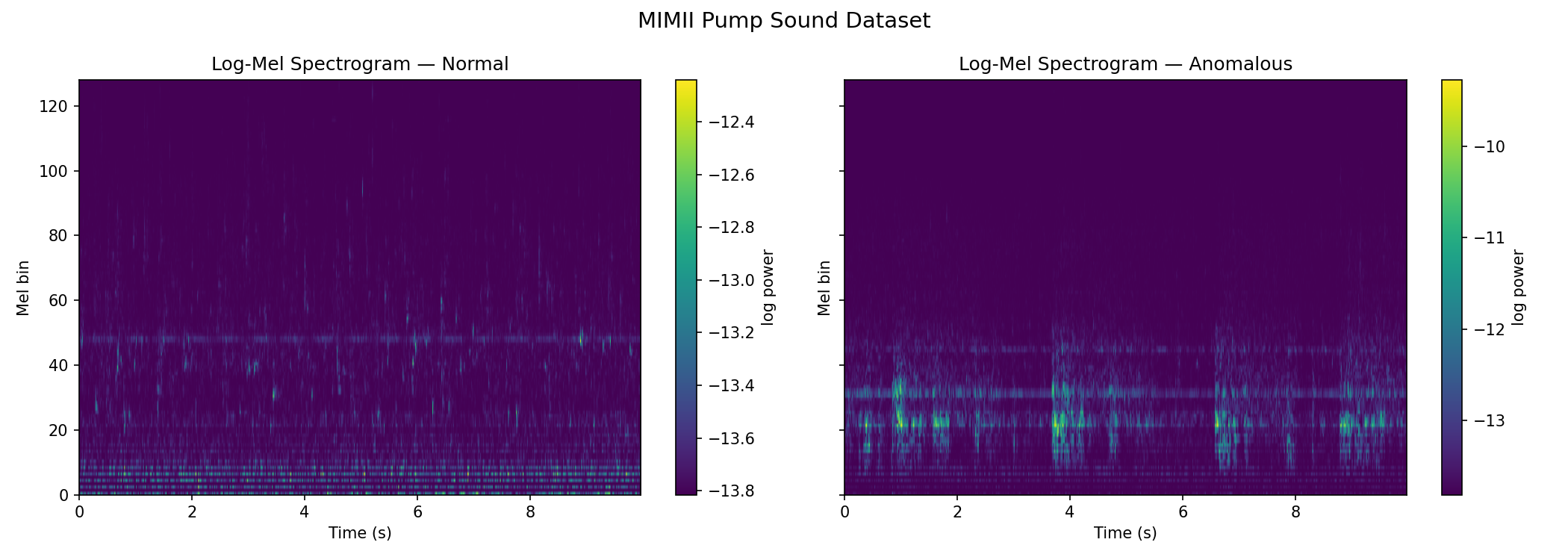 Log mel spectrograms, normal (left) vs anomalous (right), MIMII pump dataset.
The visual difference is subtle; the anomaly information is carried in the
statistical structure of the representation, not its gross appearance.
Log mel spectrograms, normal (left) vs anomalous (right), MIMII pump dataset.
The visual difference is subtle; the anomaly information is carried in the
statistical structure of the representation, not its gross appearance.
All preprocessing is implemented from scratch in NumPy/SciPy, without librosa. This keeps the pipeline transparent and removes a dependency that often introduces subtle version dependent differences.
2. First experiment: Dense AE vs TransformerVAE on a single machine type
The first dataset is the MIMII pump dataset (Purohit et al., 2019): a single machine type (pump), approximately 380 normal and 136 anomalous clips at 16 kHz, 10 seconds each. This is a controlled setting (one machine type, no machine ID variation) that isolates the core question: can a model trained on normal sounds flag anomalies at test time?
2.1 Dense Autoencoder
An Autoencoder (AE) encodes a flattened log mel spectrogram through a low dimensional bottleneck and reconstructs the input. Trained on normal sounds only, the intuition is that the reconstruction manifold covers the space of normal acoustic patterns. An anomalous clip, lying outside this manifold, should produce higher reconstruction error:
\[\text{score}_\text{AE}(x) = \frac{1}{D}\|x - \hat{x}\|^2\]The Dense AE here has ~0.9 M parameters and takes the full flattened spectrogram (8,192 dimensions) as input.
2.2 TransformerVAE
A Variational Autoencoder (VAE) extends the AE with a probabilistic bottleneck. Instead of encoding $x$ to a point, the encoder outputs the parameters of a Gaussian distribution $q_\phi(z|x) = \mathcal{N}(\mu, \boldsymbol{\Sigma})$, where $\boldsymbol{\Sigma} = \mathbb{E}[(X-\mu)(X-\mu)^T]$ is the covariance matrix (Do, 2008) and the encoder’s independence assumption across latent dimensions gives the diagonal form $\boldsymbol{\Sigma} = \text{diag}(\sigma^2)$. A sample $z = \mu + \sigma \odot \varepsilon$, $\varepsilon \sim \mathcal{N}(0, I)$ is passed to the decoder. Training maximizes the Evidence Lower Bound (ELBO):
\[\log p(x) \ge \underbrace{\mathbb{E}_{q_\phi(z|x)}[\log p_\theta(x|z)]}_{\text{reconstruction}} - \underbrace{D_\text{KL}(q_\phi(z|x) \| \mathcal{N}(0,I))}_{\text{KL regularization}}\]The anomaly score is the negative ELBO:
\[\text{score}_\text{VAE}(x) = \|x - \hat{x}\|^2 + \beta\, D_\text{KL}\]Here the encoder and decoder are Transformer blocks (Vaswani et al., 2017) operating on 2D log mel patches, using the same Multi Head Attention mechanism defined in From Keywords to Semantics applied to spectral patches instead of token sequences. The model has ~1.4 M parameters.
2.3 Results: VAE beats the AE, and the KL term is why
The results below are evaluated over 5 random seeds; AUROC is the primary metric (chance = 0.500).
| Model | AUROC | pAUC@0.1 |
|---|---|---|
| PCA baseline | 0.703 ± 0.004 | 0.663 ± 0.004 |
| Dense AE | 0.708 ± 0.004 | 0.666 ± 0.004 |
| TransformerVAE (reconstruction only) | 0.710 ± 0.004 | N/A |
| TransformerVAE (full ELBO) | 0.775 ± 0.015 | 0.651 ± 0.004 |
pAUC@0.1: partial AUC normalized to [0,1] over the false positive rate range [0, 0.1], the DCASE standard metric for low FPR operating points.
The VAE advantage is statistically significant on all 5 seeds (DeLong paired test, $p < 0.001$ each). The important finding is where the signal comes from: the KL term separates normal and anomalous clips more cleanly than the reconstruction error alone. The probabilistic bottleneck assigns tighter posteriors (higher KL) to anomalous sounds, even when the reconstruction error does not obviously increase.
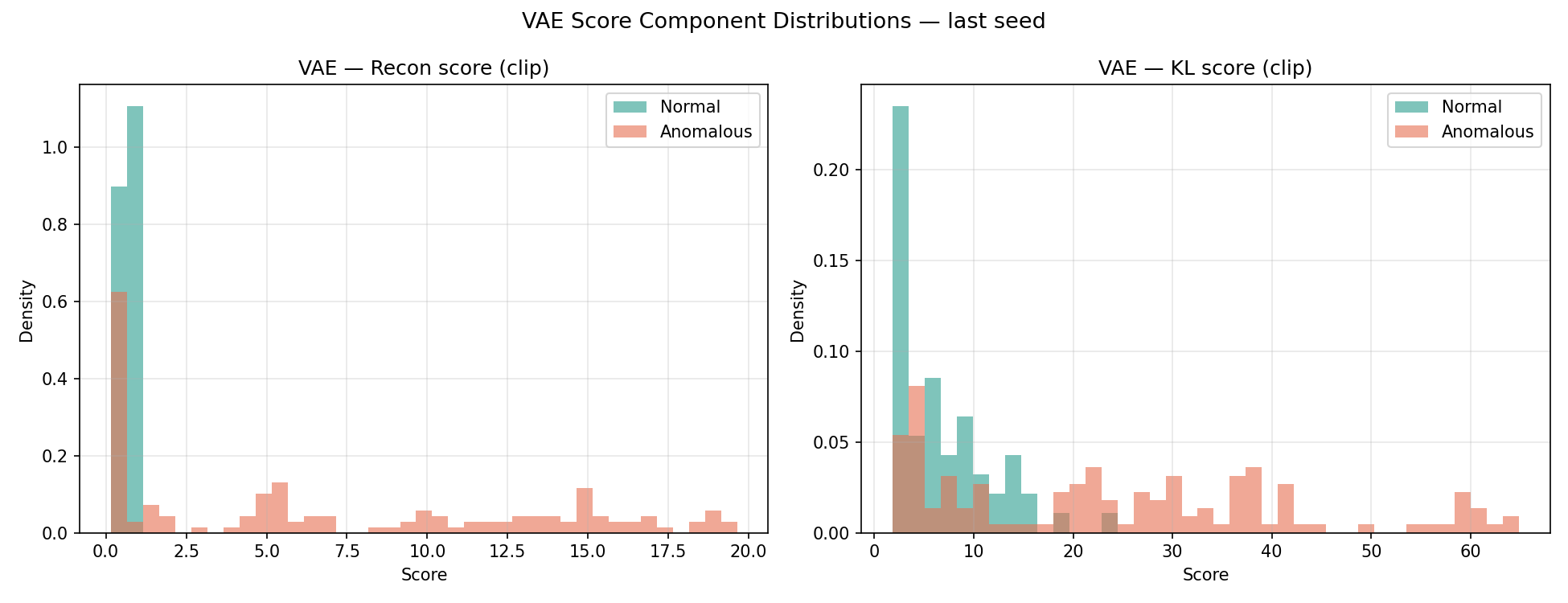 Score distributions for normal (green) and anomalous (orange) pump clips.
Left: VAE reconstruction score. Right: KL divergence score. The KL term
separates the two distributions more cleanly than reconstruction error alone.
Score distributions for normal (green) and anomalous (orange) pump clips.
Left: VAE reconstruction score. Right: KL divergence score. The KL term
separates the two distributions more cleanly than reconstruction error alone.
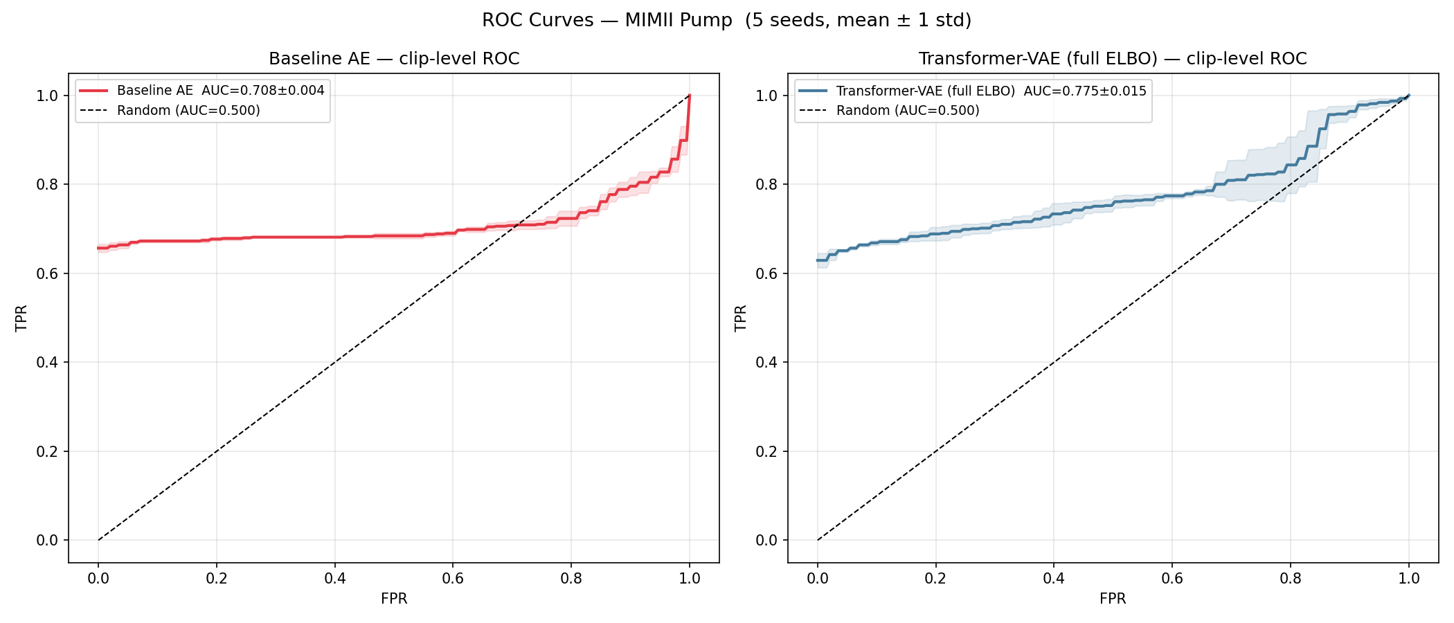 ROC curves for all models on the MIMII pump dataset, mean ± 1 std across
5 seeds. The TransformerVAE (full ELBO) curve lies consistently above the
others, particularly at low false positive rates.
ROC curves for all models on the MIMII pump dataset, mean ± 1 std across
5 seeds. The TransformerVAE (full ELBO) curve lies consistently above the
others, particularly at low false positive rates.
The Dense AE and the reconstruction only VAE are essentially tied: the Transformer architecture in the VAE encoder does not itself drive the improvement. The improvement comes from the probabilistic bottleneck and the KL term as an anomaly signal.
3. Scaling up: DCASE 2020 Task 2
The DCASE 2020 Task 2
dataset (Koizumi et al., 2020) is more demanding. It covers three machine types (fan, pump, and valve),
each recorded at 0 dB signal to noise ratio (the hardest condition), with four
physical machine units per type (IDs id_00, id_02, id_04, id_06). The
official evaluation metric is per machine ID mean AUROC: AUC computed
separately for each physical unit, then averaged across units and seeds.
This change in evaluation protocol matters. A model that confuses the normal sound signatures of different machine IDs will artificially inflate its AUC when scores are pooled; the per ID metric removes that artifact and forces the model to discriminate anomalies within each unit’s normal distribution.
3.1 Reconstruction based models hit a ceiling
Running the same AE and TransformerVAE families on DCASE 2020 reveals a sharp limitation:
| Detector | Fan | Pump | Valve |
|---|---|---|---|
| Dense AE | 0.501 ± 0.000 | 0.671 ± 0.000 | 0.632 ± 0.003 |
| TransformerVAE (KL) | 0.491 ± 0.010 | 0.631 ± 0.007 | 0.439 ± 0.065 |
| TransformerVAE (recon) | 0.501 ± 0.000 | 0.667 ± 0.001 | 0.591 ± 0.055 |
On fan, both models score 0.501 (chance). Fan anomalies produce subtle frequency domain shifts that do not change reconstruction error in any measurable way: the dominant broadband fan noise is reconstructed at low MSE even for a faulty clip, because most of the acoustic content is perfectly normal. On valve, the VAE KL score actually inverts (0.439 < 0.500): the KL regularization destroys the inter ID structure that would otherwise be useful.
This is the ceiling of reconstruction based anomaly detection: it works when faults manifest as something globally different from the reconstruction manifold, and fails when the fault signature is fine grained or machine ID specific.
4. The embedding approach: a pretext task and Mahalanobis distance
The failure on fan motivates a different question during training. Instead of asking “can the model reconstruct this clip?”, we ask: “can the model identify which physical machine this clip came from?”
This is a pretext task: a supervised objective chosen not because the
classification itself is useful at deployment, but because solving it forces
the encoder to learn fine grained acoustic signatures. A pump with ID id_00
sounds subtly different from one with id_02; learning to tell them apart
requires the model to represent the specific acoustic identity of each unit
during normal operation.
The architecture is an encoder only Transformer (no decoder, no reconstruction):
\[\text{wav} \xrightarrow{\text{STFT + mel}} S \in \mathbb{R}^{T \times F} \xrightarrow{\text{patches}} \{p_i\}_{i=1}^{P} \xrightarrow{f_\theta} \mathbf{H} \in \mathbb{R}^{P \times d} \xrightarrow{\text{GAP}} \mathbf{e} \in \mathbb{R}^d \xrightarrow{\text{classification head}} \hat{y}\]where $P = 8$ nonoverlapping patches of $N_\text{frames} = 8$ frames each, $d = 128$, and GAP is Global Average Pooling. Sinusoidal positional encoding is added before the Transformer layers. The classification head is trained with cross entropy over machine IDs.
After training, the classification head is discarded, exactly as the MLM head is discarded in language model pretraining (see From Keywords to Semantics). What remains is a 128 dimensional embedding that encodes the acoustic identity of the machine.
4.1 From the stationary distribution of a diffusion process to Mahalanobis distance
To understand why Mahalanobis distance is the right anomaly score here, it helps to derive it from the probability density function of the normal operation embedding distribution, and that derivation connects directly to the physics of stochastic processes.
Consider a machine operating normally. Its embedding $\mathbf{z} \in \mathbb{R}^d$ is a random variable whose fluctuations around the mean $\boldsymbol{\mu}_k$ can be modelled as an anisotropic diffusion process. The Langevin equation in $d$ dimensions is:
\[\dot{\mathbf{z}} = -(\mathbf{z} - \boldsymbol{\mu}_k) + \boldsymbol{\eta}(t)\]where $\boldsymbol{\eta}(t)$ is a $d$ dimensional Gaussian white noise with:
\[\langle \eta_i(t) \rangle = 0, \qquad \langle \eta_i(t)\,\eta_j(t') \rangle = 2D_{ij}\,\delta(t - t')\]The tensor $\mathbf{D} \in \mathbb{R}^{d \times d}$ is the diffusion coefficient matrix: it encodes how strongly the process fluctuates in each direction and how those fluctuations are correlated across dimensions. For isotropic noise $\mathbf{D} = D\mathbf{I}$; in general $\mathbf{D}$ is symmetric positive definite.
Starting from a known initial state $\mathbf{z}_0$ at time $t_0$, this Langevin equation determines a conditional, or transition, probability density function $P(\mathbf{z}, t \mid \mathbf{z}_0, t_0)$ for where the embedding is likely to be found at a later time $t$. To lighten the notation, we write the probability density function as $P(\mathbf{z}, t)$.
The Fokker–Planck equation governing the time evolution of this probability density function is:
\[\frac{\partial P}{\partial t} = \nabla \cdot \bigl[(\mathbf{z} - \boldsymbol{\mu}_k)\,P\bigr] + \nabla \cdot \mathbf{D}\,\nabla P\]As $t \to \infty$, setting $\partial P / \partial t = 0$ gives the stationary solution. For this linear drift with anisotropic diffusion, the stationary solution is a multivariate Gaussian:
\[p_s(\mathbf{z}) = \frac{1}{(2\pi)^{d/2}\,|\boldsymbol{\Sigma}_k|^{1/2}} \exp\!\left(-\frac{1}{2}(\mathbf{z} - \boldsymbol{\mu}_k)^\top \boldsymbol{\Sigma}_k^{-1} (\mathbf{z} - \boldsymbol{\mu}_k)\right)\]where the covariance matrix is related to the diffusion tensor by the fluctuation dissipation relation:
\[\boldsymbol{\Sigma}_k = \mathbf{D}\]This is the key identity: the covariance matrix of the stationary distribution is exactly the diffusion coefficient matrix. Directions in which the process diffuses weakly (small eigenvalues of $\mathbf{D}$) correspond to tightly clustered embeddings (small eigenvalues of $\boldsymbol{\Sigma}_k$). The precision matrix $\boldsymbol{\Sigma}_k^{-1}$ is proportional to the inverse diffusion tensor: it encodes the stiffness of the process in each direction.
The negative log likelihood of the stationary distribution is:
\[-\log p_s(\mathbf{z}) = \frac{1}{2}(\mathbf{z} - \boldsymbol{\mu}_k)^\top \boldsymbol{\Sigma}_k^{-1} (\mathbf{z} - \boldsymbol{\mu}_k) + \text{const}\]and the argument of the exponential is exactly $\frac{1}{2}d_\text{Maha}^2$, where:
\[d_\text{Maha}(\mathbf{z}, k) = \sqrt{(\mathbf{z} - \boldsymbol{\mu}_k)^\top \boldsymbol{\Sigma}_k^{-1} (\mathbf{z} - \boldsymbol{\mu}_k)}\]The Mahalanobis distance is the negative log likelihood of the embedding under the stationary distribution of the normal operation process. Scoring anomalies by Mahalanobis distance is equivalent to asking: how unlikely is this embedding under the fitted multivariate Gaussian, or, in the Langevin picture, how far has the system drifted from its stationary state?
The physical intuition is direct. A machine operating normally generates embeddings that fluctuate around $\boldsymbol{\mu}_k$ with covariance $\boldsymbol{\Sigma}_k$, the fingerprint of its normal acoustic behavior. A fault perturbs the process, pushing the embedding outside the stationary distribution. The Mahalanobis distance measures the magnitude of that perturbation relative to the natural fluctuation amplitude in each direction of the embedding space, weighted by the inverse diffusion tensor.
In practice, $\boldsymbol{\Sigma}_k$ is estimated from the training embeddings using Ledoit–Wolf shrinkage (Ledoit & Wolf, 2004), which regularizes the sample covariance matrix toward a scaled identity, essential for numerical stability when the number of training clips is not large compared to the embedding dimension $d = 128$.
At inference, with no known machine ID, the score is the minimum negative log likelihood over all IDs:
\[d_\text{auto}(\mathbf{z}) = \min_k \; d_\text{Maha}(\mathbf{z}, k)\]An anomalous clip should sit far from all stationary distributions simultaneously, unlikely under every machine’s normal operation model.
4.2 ArcFace: tightening the clusters on the hypersphere
How well the Mahalanobis approach works depends on the geometry of the learned embedding space. With a standard softmax cross entropy head, embeddings of the same machine ID can point in very different directions: the model only needs to be linearly separable across IDs, not compactly clustered. Loose clusters produce imprecise precision matrices and allow anomalous embeddings to drift close to the centroid of the wrong ID under the autoselect minimum distance scoring.
ArcFace (Deng et al., CVPR 2019) addresses this by training directly on the hypersphere. Both embeddings and classification weight vectors are L2 normalized, and an additive angular margin $m$ is imposed on the target class angle $\theta_y$ before the softmax:
\[\mathcal{L}_\text{ArcFace} = -\log \frac{e^{s \cos(\theta_y + m)}}{e^{s \cos(\theta_y + m)} + \sum_{k \neq y} e^{s \cos \theta_k}}\]with $s = 32$, $m = 0.10$ radians. The margin forces each embedding toward its class prototype throughout training, not just enough to beat the competing IDs, but enough to clear the angular margin. Clusters tighten, the precision matrices become more faithful representations of the local normal geometry, and autoselect scoring becomes reliable without a known machine ID at inference.
4.3 A modality specific correction
One additional finding is worth noting. Applying random time and frequency masking (SpecAugment, Park et al., 2019) during training improved detection on fan but caused a large regression on valve. Valve faults produce strong, localized spectral signatures at specific frequency bands; training the encoder to be robust to missing frequency bands trains it to ignore precisely those signatures. The fix is per type: fan and pump use full augmentation; valve disables it. The right augmentation strategy depends on where the signal lives, not on a uniform recipe.
5. Full results
The per machine ID mean AUROC across all three detector families:
| Detector | Fan | Pump | Valve |
|---|---|---|---|
| Dense AE | 0.501 ± 0.000 | 0.671 ± 0.000 | 0.632 ± 0.003 |
| TransformerVAE (reconstruction) | 0.501 ± 0.000 | 0.667 ± 0.001 | 0.591 ± 0.055 |
| TransformerVAE (KL) | 0.491 ± 0.010 | 0.631 ± 0.007 | 0.439 ± 0.065 |
| Embedding + Mahalanobis (oracle per ID) | 0.714 ± 0.012 | 0.645 ± 0.015 | 0.966 ± 0.009 |
| Embedding + Mahalanobis + ArcFace (autoselect) | 0.730 ± 0.005 | 0.738 ± 0.017 | 0.947 ± 0.006 |
Oracle per ID: machine ID known at inference. Autoselect: minimum Mahalanobis over all IDs, no machine ID required. Averaged over seeds 0, 1, 2. Chance = 0.500.
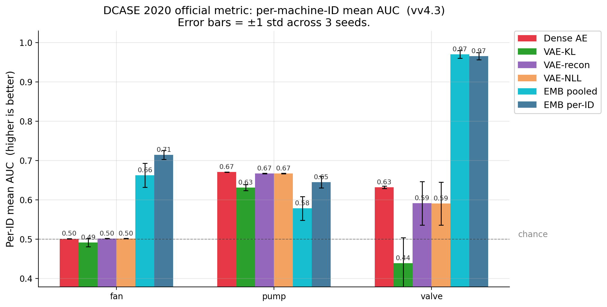 Per machine ID mean AUROC for all detector families across fan, pump, and
valve. The embedding model dominates on valve (0.966) and fan (0.714); the Dense
AE leads on pump (0.671).
Per machine ID mean AUROC for all detector families across fan, pump, and
valve. The embedding model dominates on valve (0.966) and fan (0.714); the Dense
AE leads on pump (0.671).
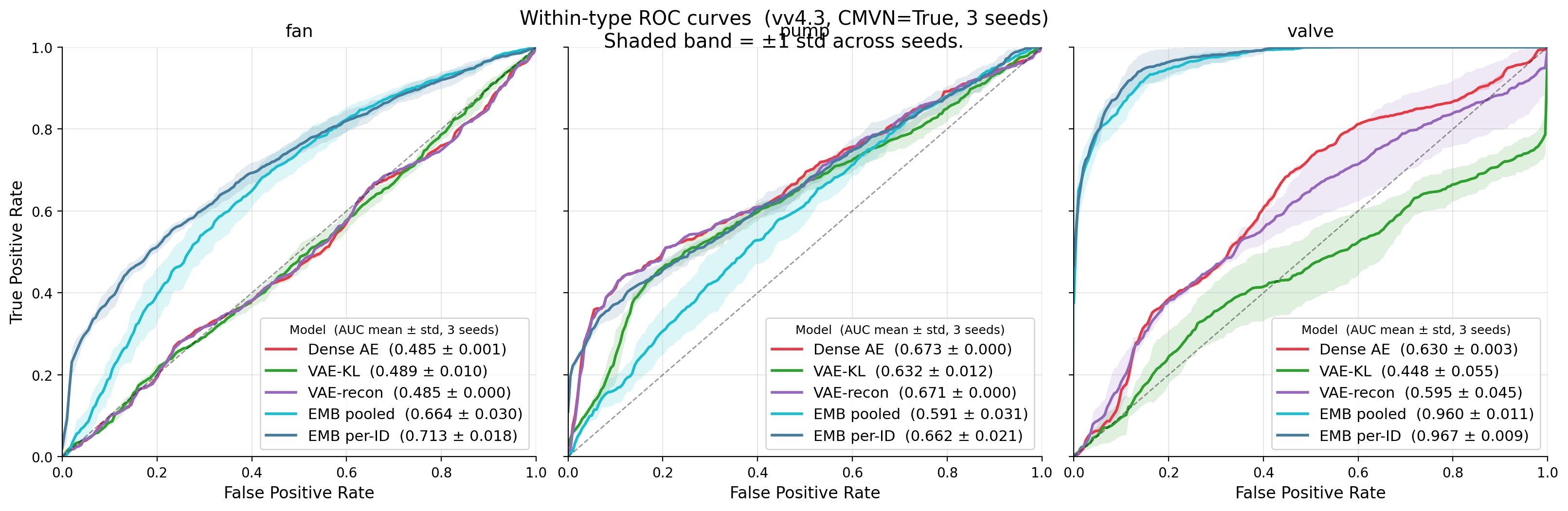 Within type ROC curves (mean ± 1 std across seeds). The embedding model
achieves a near perfect curve on valve; reconstruction based models are near the
diagonal on fan.
Within type ROC curves (mean ± 1 std across seeds). The embedding model
achieves a near perfect curve on valve; reconstruction based models are near the
diagonal on fan.
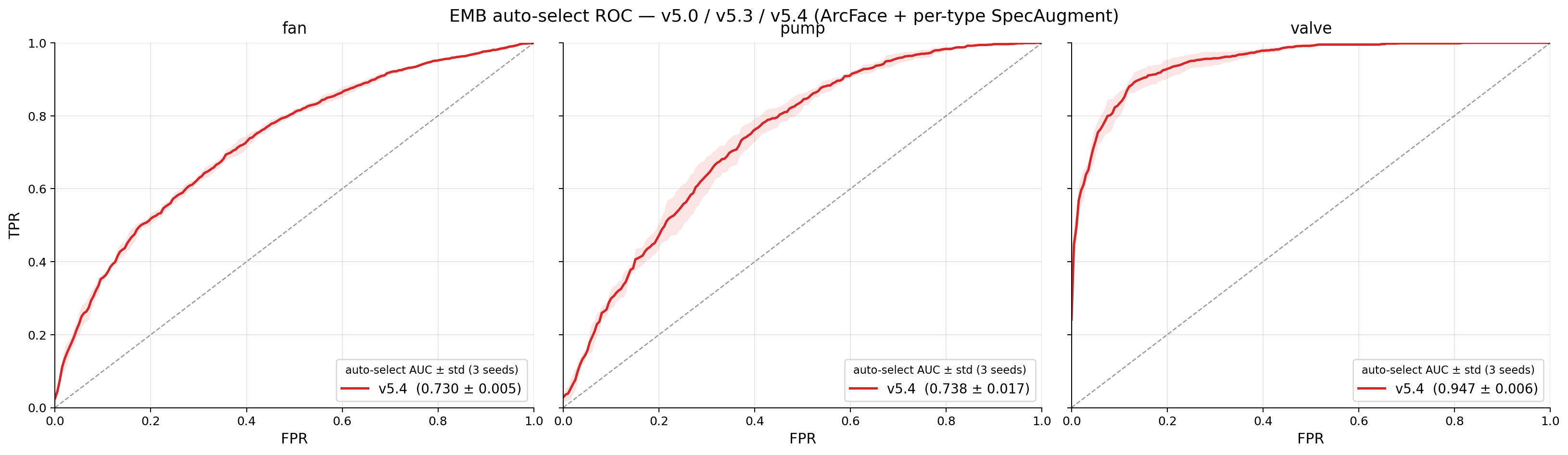 ROC curves comparing softmax CE (oracle per ID) vs ArcFace (autoselect) on
valve. The ArcFace autoselect curve closely tracks the oracle curve, 0.947 AUC
vs 0.966 AUC: most of the detection performance is recovered without the
deployment constraint of a known machine ID.
ROC curves comparing softmax CE (oracle per ID) vs ArcFace (autoselect) on
valve. The ArcFace autoselect curve closely tracks the oracle curve, 0.947 AUC
vs 0.966 AUC: most of the detection performance is recovered without the
deployment constraint of a known machine ID.
Three findings stand out. Reconstruction based models are competitive on pump but collapse to chance on fan: some fault signatures simply do not change reconstruction error. The embedding approach reverses this on fan and achieves near perfect detection on valve. The ArcFace loss makes autoselect scoring practical across all three machine types (0.730, 0.738, and 0.947 AUC on fan, pump, and valve), coming within a few points of the oracle score on valve (0.966), so the system can be deployed without knowing which physical unit the recording came from.
5.1 A pooled view and the low FPR metric
The per machine ID metric evaluates each physical unit’s normal distribution separately, then averages. A complementary evaluation pools all clips within a machine type together, ignoring the per unit structure, and also reports pAUC@0.1, the low false positive rate metric introduced in Section 2. It also gives a natural way to ablate the embedding model itself: score against a single Gaussian fit on all training embeddings pooled across machine IDs, instead of the per ID Gaussians used by the oracle scorer.
| Detector | Fan AUC | Fan pAUC@0.1 | Pump AUC | Pump pAUC@0.1 | Valve AUC | Valve pAUC@0.1 |
|---|---|---|---|---|---|---|
| Dense AE | 0.485 ± 0.001 | 0.044 ± 0.000 | 0.673 ± 0.000 | 0.276 ± 0.001 | 0.630 ± 0.003 | 0.063 ± 0.001 |
| TransformerVAE (KL) | 0.489 ± 0.010 | 0.043 ± 0.001 | 0.632 ± 0.012 | 0.127 ± 0.020 | 0.448 ± 0.055 | 0.051 ± 0.023 |
| TransformerVAE (recon) | 0.485 ± 0.000 | 0.043 ± 0.000 | 0.671 ± 0.000 | 0.272 ± 0.001 | 0.595 ± 0.045 | 0.083 ± 0.029 |
| Embedding + Mahalanobis (pooled Gaussian) | 0.664 ± 0.030 | N/A | 0.591 ± 0.031 | N/A | 0.960 ± 0.011 | N/A |
| Embedding + Mahalanobis (oracle per ID) | 0.713 ± 0.018 | 0.273 ± 0.024 | 0.662 ± 0.021 | 0.293 ± 0.016 | 0.967 ± 0.009 | 0.771 ± 0.013 |
Pooled across all clips within a machine type rather than averaged per machine ID. pAUC@0.1: partial AUC over the false positive rate range [0, 0.1]. pAUC@0.1 is not computed for the pooled Gaussian ablation.
On valve and fan, pooled AUC and per machine ID mean AUC agree closely (0.967 vs 0.966 on valve, 0.713 vs 0.714 on fan), so the oracle embedding model’s ranking holds under either evaluation protocol. On pump, Dense AE remains the strongest detector under both metrics (0.673 pooled vs 0.671 per machine ID), consistent with the earlier finding that Dense AE, not the embedding model, leads on pump. The pAUC@0.1 gap is the largest signal in the whole results set: 0.771 for the oracle embedding model on valve against 0.051 to 0.083 for the reconstruction based models, meaning the embedding model stays reliable specifically at the low false positive rate operating points that matter for deployment, not only in aggregate AUC.
Ignoring the per machine ID structure entirely, by scoring against one Gaussian fit on all training embeddings pooled across IDs, costs real detection performance on fan (0.664 vs 0.713) and pump (0.591 vs 0.662), and is essentially unchanged on valve (0.960 vs 0.967). The per ID means and covariances derived in Section 4.1 capture structure a single global Gaussian cannot: on valve the fault signature is already strong enough that almost any Gaussian catches it, but on fan and pump the per ID structure is doing real work, which is exactly why ArcFace autoselect (Section 4.2), which keeps that per ID structure without requiring a known ID at inference, is worth the added training complexity.
6. What ties this back to retrieval
In RAG as a Hilbert Space Problem, cosine similarity on the unit hypersphere is the natural retrieval metric because there is no prior knowledge about the distribution of documents in embedding space: you know nothing about its covariance structure, so angle is all you have. In the anomaly detection setting, that prior knowledge exists: the full stationary distribution of normal embeddings is available from training, fitted as a multivariate Gaussian whose covariance is proportional to the diffusion tensor of the underlying acoustic process. Mahalanobis distance is the negative log likelihood of that distribution, the physically motivated metric that cosine cannot recover without knowing the covariance.
ArcFace closes the loop: by training on the hypersphere with an angular margin loss, it produces the tight per machine clusters that make the fitted Gaussian a faithful model of the stationary distribution, and Mahalanobis autoselection reliable without a known machine ID at inference.
The architecture throughout is the same encoder only Transformer. The modality is different. The distance metric differs because the information available at inference time differs, and that information has a precise physical meaning as the covariance of a stationary diffusion process. That is the complete story.
References
- Deng, J., Guo, J., Xue, N., & Zafeiriou, S. (2019). ArcFace: Additive Angular Margin Loss for Deep Face Recognition. CVPR.
- Do, C. B. (2008). The Multivariate Gaussian Distribution. CS229 Section Notes, Stanford University. https://cs229.stanford.edu/section/gaussians.pdf
- Koizumi, Y., et al. (2020). DCASE 2020 Task 2: Unsupervised Anomalous Sound Detection for Machine Condition Monitoring. DCASE Workshop.
- Ledoit, O., & Wolf, M. (2004). A well-conditioned estimator for large-dimensional covariance matrices. Journal of Multivariate Analysis.
- Park, D. S., Chan, W., Zhang, Y., et al. (2019). SpecAugment: A Simple Data Augmentation Method for Automatic Speech Recognition. Interspeech.
- Purohit, H., Tanabe, R., Ichige, T., Endo, T., Nikaido, Y., Suefusa, K., & Kawaguchi, Y. (2019). MIMII Dataset: Sound Dataset for Malfunctioning Industrial Machine Investigation and Inspection. DCASE Workshop.
- Stevens, S. S., Volkmann, J., & Newman, E. B. (1937). A Scale for the Measurement of the Psychological Magnitude Pitch. Journal of the Acoustical Society of America, 8(3), 185–190.
- Vaswani, A., et al. (2017). Attention is all you need. NeurIPS.